The solar rotation rate
from inversion of the first GONG datasets
- Abstract ; References
- Basic equations
- Selected GONG datasets
- L-curves: A guide for the choice of trade-off parameters ?
- A solution with dataset I and L-curves based choice for the trade-off parameters
- How sharp is the transition zone ? Results of inversions with less regularization
- Results from dataset II and Preliminary works on
the introduction of a discontinuous Basis of B-splines
Th.Corbard, G. Berthomieu, J. Provost.
Laboratoire G.-D.Cassini, Observatoire de la Côte d'Azur, Nice.
This poster gives some results obtained by inverting GONG datasets for the rotational splittings with a full 2D regularized least square method. This technique is based on a projection of the rotation on a tensorial product of B-splines, and could be very powerful to reach some fine information without increasing too much the number of variables.
A generalization to the 2D problem of the so-called L-curves is discussed and used as a guide for the choice of trade-off parameters.
The GONG months 4 to 8 datasets including both averaged (for degrees up to l=150) and concatenated (for degrees lower than l=30) spectra are inverted and discussed. The resolution of the inversion is studied using averaging kernels leading to an upper limit for the transition zone at the base of the convective zone.
The last available data from averaged spectra of GONG months 4 to 10 are inverted too. For this dataset, preliminary works on the introduction of a discontinuous basis of B-splines is presented.
References:
Christensen-Dalsgaard, J. & Berthomieu, G. 1991, in Solar Interior and Atmosphere,
ed. A.N.Cox, W.C. Livingstone, & M. Matthews (Tuscon: Univ. of Arizone Press), 401.
T.Corbard, G. Berthomieu, G. Gonczi, J. Provost, P. Morel, 1995, Fourth Soho Workshop,
Helioseismology, esa sp-376, 289-294.
Hansen, C., 1992, Numerical tools for analysis and solution of Fredholm integral
equations of first kind, Inverse Problems 8: 849-872.
Ritzwoller M.H., Lavely E.M., 1991, ApJ 369, 557
Schou, J., Christensen-Dalsgaard, J. & Thompson, M.J. 1994, On comparing helioseismic
two-dimmensional inversion methods, ApJ, 433: 389-416
Snodgrass, H.B., 1984, Solar phys., 94, 13.
An observable consequence of the solar rotation is that frequencies of solar oscillation
modes (n,l,m) are splitted in a m multiplet. for low rotation the frequency shifts are
given by:
where
We search for the unknown rotation as a linear combination of piecewise polynomials,
projected on a tensorial product of B-spline basis (Corbard et al., 1995). We take into
account the observational
errors (with standard deviation
The regularization parameters
The inversion depends on the number of piecewise polynomials, on the order of the spline
functions and on the distribution of the break points of these polynomials. In what follows, the distribution of these points along the radius has been chosen according to the density of the turning
points of the considered p-modes for a given dataset.
The inferred rotation
The radial and latitudinal full widths at mid height (
We present the solutions obtained for two differents datasets.
The second dataset (data II) has been obtained from averaged spectra of GONG months
4 to 10 for degrees
In both cases individual splittings and their corresponding errors have been calculated
from their expansion on polynomials and inversions have been performed from these
individual splittings.
A guide for the choice of the trade-off parameters
One can plot the value of each part of the regularization term against the
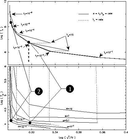
This figure shows an example of such L-curves obtained for dataset I and with
second derivative (i=2) in the regularization term in radius (
The upper figure shows the logarithm of the value of the regularization term
The full curves join points with the same ratio
On the lower figure the value of the logarithm of the regularization term
According to these two figures, a choice like point 1 on the figure (
When a regularization term in latitude
L-curves reveal themself as being an useful tool to study the variation
and mutual dependencies of each term in Eq.(4)
for different choices of trade-off parameters and functions
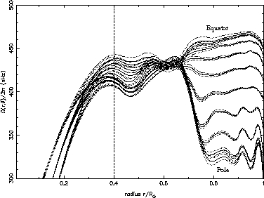
The inferred rotation rate is shown as a function of radius for ten latitudes from
the equator
up to the pole (
Below
In the whole convection zone the rotation rate presents
the same latitudinal variation as at the surface
with a positive gradient just beneath the surface for latitude from the equator up to
Dotted curves represent the
These figures show contour plots of the averaging kernels at solar pole, mid
latitude and equator for
At
The radial resolution at the base of the convection zone (
This inferred rotation rate has a sharper transition zone than the previous
one (about
At
At 0.4
The possibility of introducing a discontinuous basis of B-splines might give a
test of the reliability of the inferred rotation rate at a target radius. The idea is to
allow the rotation to be discontinuous at a given depth and to look, after inversion,
if the inferred rotation is discontinuous at this location or not. Solutions that
are physically realistic should be continuous at each point but in zones where the solution
is not well constrained such inversion could produce different values for the rotation
rate on the right and on the left of the break point. Our preliminary results show that the
gap between the right and left values is low where the solution is thought to be well
constrained by the data and larger elsewhere.
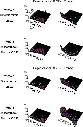
The
Averaging kernels obtained at the equator and
This work is very preliminary
and we think that numerical experiments on the reconstruction of some arbitrary given
test rotation rates
should be useful to calibrate the effect
of introducing a discontinuous basis.

 is the unperturbed mode frequency,
  is the unknown rotation rate versus depth and latitude,
 ,
,  is the colatitude and r the normalized solar radius. The kernels
  depend on the model
and the eigenfunctions of the mode which are assumed to be known exactly
(e.g. Christensen-Dalsgaard & Berthomieu 1991).
 ) and a regularization term to avoid the large
spurious variations of the solution induced by the ill-conditioned inversion problem. Thus we
search coefficients that represent the projection of the rotation rate on the chosen B-splines
basis by minimizing:


 and
and  and functions
  and
and  are used to define the trade off
between the resolution and the propagation of the input errors. We can choose any derivative
of the rotation rate. This leads to different behavior of the rotation especially at
locations where
the observed modes are not enough to constrain the solution. For the results discussed here we
choose
  , i=2 and
  with j=1,2.
 at a
point (
 ) is obtained as a linear combination of the
data
  . Thus from Eq.(1) it follows that averaging kernels
  ,
which are a linear combination of rotational kernels
  , exist such that:

 and
and
 ) of these kernels provide an estimation of the spatial resolution of the
inversion at a point
 . It increases with lower regularizing term, at the expense of larger errors on
the solution.
 diagrams show the different
modes concerned in each case.
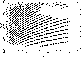
 .
Splittings are given by their expansion on Legendre polynomials with coefficients up to
  .
.
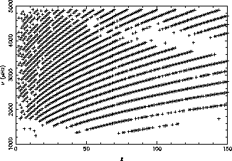
 .
It contains 2103 modes
 with
with
with
with  . Splittings are given
by their expansion on orthogonal polynomials with coefficients up to
  .
The orthogonal polynomials are defined in Ritzwoller & Lavely (1991).
 and
and  could be a generalization of the so called L-curves currently used in one dimensional problems
(Hansen, 1992).
The aim is to find parameters that minimize both the
  value obtained for the fit of observed splittings (i.e. the first term in the sum Eq.(4))
and the two regularization terms
  and
and  .
.
 value
and this for different choices of
  and
and
 . An interesting result is that in a log-log plot, for large values of the
trade off parameters the
  value gets large for little reduction of regularization terms
and, in the opposite, for small values of lambdas the regularization terms get large for small
reduction of the
  value. Reasonable choices of trade-off parameters are therefore
those in the vicinity of the corner of the L-curve.
 ) and
first derivative (j=1) in
  .
.
 against
 where N is the total number of splittings, this for different values
of
  and
and  . One can see that all the points
on this figure which are labeled by the same
  but different
  have the
same location except for very large values of
  (i.e.
(i.e.  ) .
Thus it appears that the two terms (
 and
and  )
do not depend on the value of
  for a large domain of variation of this parameter
(
 ).
).
 . According to the previous discussion, on the upper
figure all these curves reduce to
only one if we do not look at solutions obtained with
  that are too much
regularized.
 is plotted against
  for six values of the ratio
 . As
. As  decreases the
position of the L-curve becomes lower showing that for a given value of
  ,
the
,
the  value must be as large as possible (always with the limitation
  )
if one wants to reduce the value of the regularization term in latitude.
 ,
,  , i.e.
 ) tends to minimize both the
  value and the two regularization
terms.
 is chosen with second derivative (j=2), the
corresponding
plots have similar behaviors but the domain of variation for
  , for which
  and
and
 depend only on
  , is smaller (
 .
.
 and
and  .
Nevertheless other methods for the optimal choice of trade-off parameters are possible.
In particular, for a local estimation of the quality of the solution, we must have a look at
the balance between the effect
of propagating input errors
and the resolution reached at a target location
  .
.
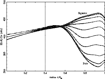
 ). This solution
is very smooth and has no latitudinal dependence below 0.6 solar radius.
 the
solution is not reliable because of the lack of modes able to describe these depths leading
to averaging kernels that are large, not well localized and that consist in several peaks.
The latitudinal independence found for these depths results essentially from the choice
of j=1 in the regularization term
  . This choice could be judicious for an attempt
to sound the very deep interior from such global inversion, without searching for
a description of a latitudinal dependence in the core that should require very low errors in data.
Nevertheless, our current investigations and the averaging kernels that we obtained
do not allow us to draw an inference from the solution obtained below
  .
.
 .
The transition to a latitudinal independent rotation in the radiative zone occurs between
0.8 and 0.6 solar radius for latitude up to
  .
.
 errors on the solution which are
the result of propagating input errors on the splittings through the inversion. In this inversion
these errors
are very low because the regularization is very strong. In fact
these errors represent the difference between the inferred rotation and the true
rotation rate convolved with the averaging kernels as in Eq.(5).(see e.g. Schou et al 1994).
A look at these kernels is needed
to qualify the resolution of the inversion.
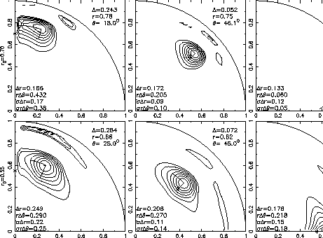
 .
.  is the geometrical distance
between position
  of the maximum value of the averaging kernel and the point
(
 ) shown as a star on figures.
This quantity is very high for averaging kernels calculated near the pole (
 ),
showing that for these latitudes we are not able to obtained well peaked kernels and
inferred the solution
is not reliable.
 the estimated rotation rate is latitudinal independent. Nevertheless
the latitudinal resolution at
  is very low (
 at
mid latitude) and could produce a smoothing
effect on a latitudinal variation if any exists.
 ) is around
 at mid latitude and is almost as large as the transition observed on the solution
(
 ). Thus if the transition is sharper this inversion doesn't enable to
resolve it. Inversions with less regularization have been performed to study this
transition zone.
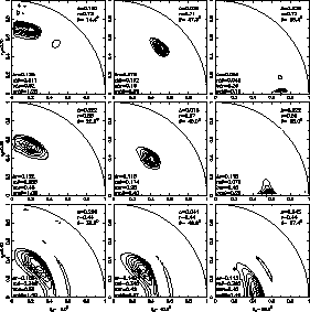
 , i=2 and
 , j=1 and the corresponding averaging kernels for
  and
and  . This choice of trade-off parameters, (shown as
the point 2 on L-curves figure)
tends to minimize the
  value rather
than the two regularization terms. This leads to a solution with some oscillations especially
in zones near the solar pole where the solution is not well constrained by the data.
 ) and the averaging kernels at this location (
 ) are
better peaked with an increasing radial resolution (
 at mid latitude).
Inversion performed with lower regularization doesn't enable to produce better radial resolution
and increase the effect of input errors, leading to an increasing product
  .
Thus, this
inversion is the one that gives the best radial resolution at this target location without increasing to much the effect of input errors.
The fact that the width of the transition zone decreases when
the resolution increases allows us to say that the transition occurs in a zone between
0.66 and 0.76 solar radius but it might be sharper than this.
 averaging kernels at
  and
and  are, for this inversion,
sufficiently well localized in latitude so that the latitudinal independence of the inferred
rotation rate at
this depth can be considered as real.
 the large extent in latitude of the averaging kernels should
produce a smoothing effect i.e. almost the same averaged rotation rate for all latitudes.
Nevertheless, the solution shows again a latitudinal dependence between 0.55 and 0.35
  .
This might argues in favor of the existance of a variation with the latitude at these
depths but we are still studying how to read our results there:
some contributions in averaging kernels generated by a lack of cancelation of rotational kernels
near the surface are suspected and may explain this behavior of the inferred rotation rate in this
kind of inversion with low regularization. Moreover this latitudinal dependence below
 is of lower importance with dataset II.
 . The choice of trade-off parameters
correspond to the point 2 on the L-curves figure. The inferred rotation
rate is in good agreement with the previous one for latitudes below
  and is less oscillating near the pole. As the observed modes and the
trade-off parameters are the same as for dataset I, we can think that these
zones are now better constrained by the data. Nevertheless we can not exclude
that the regularization acts not exactly by the same way on the two datasets
so that the regularization could be more important with dataset II.
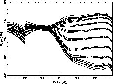
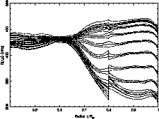
 and 0.5
 . At
. At  the solution remains continuous at the equator
and the gap
increases with the latitude up to 40 nHz at the pole.
With a discontinuous basis at 0.5
 , the gap
is around 40 nHz even
at the equator. Other results show that the gap increases again in the deep interior.
In all cases the value at the middle of the gap is equal to the value of the rotation rate that
we obtain without introducing any discontinuous basis.
Therefore this tool should provide an alternative way to estimate the error on the solution and to
show how the inversion is stable at a target location.

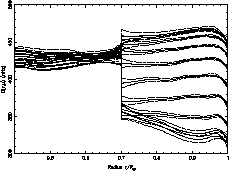
 ).
).
 value obtained
for this solution and the resolutions are almost the same than with the standard
basis indicating that data are compatible with a very sharp transition zone.
 are shown
for the solutions obtained with and without setting a discontinuous basis at
  (shown on the two transparencies).
Although, without discontinuous basis the averaging kernel was equally distributed around
 , with a discontinuous basis the major part of the kernel
is below 0.7
 . By this way the value of the rotation rate obtained at
  is less influenced by the true rotation above 0.7
 and this could explain its
lower value. This may argue in favor of a solid rotation up to
  but
this conclusion would have been more reliable if the averaging kernel had strictly no
part above
  . Furthermore the new averaging kernel is more oscillating between
 and 0.9
 so that its interpretation is harder.
A symmetrical example is shown by the averaging kernels calculated at the equator and
  with and without allowing the rotation to be discontinuous at
  . This could
explain by similar way the higher value obtained just above
  when we perform the inversion with a discontinuous basis.
Thierry Corbard
E-mail:
corbard@obs-nice.fr
Fax: (+33) 04 92 00 31 21
Dernières modifications: 16 Octobre 1996